Polars vs Pandas: A Faster DataFrame Library for Python

Maria
Python
01 Oct, 2026

pandas has been the default DataFrame library in Python for well over a decade. It's everywhere: tutorials, notebooks, data pipelines, and the APIs of half the libraries you use. Polars is the newer alternative that keeps showing up in benchmarks and on job descriptions, built in Rust, multi-threaded by default, and designed around a query engine rather than a NumPy array with labels.

The interesting question isn't which one is "better". It's what Polars does differently, whether those differences matter for your data, and what it costs you to switch. This post puts the two side by side on the same tasks, explains the ideas behind Polars (expressions and lazy evaluation), and ends with practical guidance on when each one is the right call.

The examples were run with pandas 3.0 and Polars 1.44.

Installing Both

python -m pip install pandas polars pyarrow

pyarrow isn't strictly required by Polars, but it's needed for some conversions between the two libraries and for fast Parquet support in pandas. Install everything into a project virtual environment. If you're coming to Polars from pandas basics, the Python data analysis overview covers the pandas side.

The Core Difference in One Sentence

pandas is an eager, index-based library: every operation runs immediately and returns a new object with a row index. Polars is an expression-based library with an optional lazy mode: you describe what you want as expressions, and a query engine figures out how to run them, in parallel, often skipping work it can prove is unnecessary.

Everything else follows from that. Let's see it on real code.

Same Data, Two Libraries

Here's a small orders table in Polars:

# orders.py
from datetime import date

import polars as pl

orders = pl.DataFrame(
    {
        "order_id": [1, 2, 3, 4, 5, 6],
        "customer": ["ada", "grace", "ada", "linus", "grace", "ada"],
        "region": ["EU", "US", "EU", "EU", "US", "EU"],
        "amount": [120.0, 75.5, 42.0, 310.0, 18.25, 99.9],
        "ordered_on": [
            date(2026, 9, 1), date(2026, 9, 3), date(2026, 9, 7),
            date(2026, 9, 7), date(2026, 9, 12), date(2026, 9, 20),
        ],
    }
)
print(orders)

shape: (6, 5)
┌──────────┬──────────┬────────┬────────┬────────────┐
│ order_id ┆ customer ┆ region ┆ amount ┆ ordered_on │
│ ---      ┆ ---      ┆ ---    ┆ ---    ┆ ---        │
│ i64      ┆ str      ┆ str    ┆ f64    ┆ date       │
╞══════════╪══════════╪════════╪════════╪════════════╡
│ 1        ┆ ada      ┆ EU     ┆ 120.0  ┆ 2026-09-01 │
│ 2        ┆ grace    ┆ US     ┆ 75.5   ┆ 2026-09-03 │
│ 3        ┆ ada      ┆ EU     ┆ 42.0   ┆ 2026-09-07 │
│ 4        ┆ linus    ┆ EU     ┆ 310.0  ┆ 2026-09-07 │
│ 5        ┆ grace    ┆ US     ┆ 18.25  ┆ 2026-09-12 │
│ 6        ┆ ada      ┆ EU     ┆ 99.9   ┆ 2026-09-20 │
└──────────┴──────────┴────────┴────────┴────────────┘

Two things stand out. There's no index column on the left: Polars DataFrames don't have one. And every column shows its data type under the name. Polars is strict about types: a column has exactly one type, and a native date type is used for dates rather than a generic object.

The equivalent pandas DataFrame is built the same way with pd.DataFrame({...}), and I'll call it pdf below.

Filtering and Adding Columns

In pandas, you typically filter with a boolean mask and add columns with assignment or assign:

# pandas
result = pdf[pdf["amount"] > 50].assign(
    amount_with_vat=lambda d: (d["amount"] * 1.2).round(2)
)[["customer", "region", "amount", "amount_with_vat"]]
print(result)

  customer region  amount  amount_with_vat
0      ada     EU   120.0           144.00
1    grace     US    75.5            90.60
3    linus     EU   310.0           372.00
5      ada     EU    99.9           119.88

In Polars, every transformation is a method that takes expressions, built from pl.col(...):

# polars
result = (
    orders.filter(pl.col("amount") > 50)
    .with_columns((pl.col("amount") * 1.2).round(2).alias("amount_with_vat"))
    .select("customer", "region", "amount", "amount_with_vat")
)
print(result)

shape: (4, 4)
┌──────────┬────────┬────────┬─────────────────┐
│ customer ┆ region ┆ amount ┆ amount_with_vat │
│ ---      ┆ ---    ┆ ---    ┆ ---             │
│ str      ┆ str    ┆ f64    ┆ f64             │
╞══════════╪════════╪════════╪═════════════════╡
│ ada      ┆ EU     ┆ 120.0  ┆ 144.0           │
│ grace    ┆ US     ┆ 75.5   ┆ 90.6            │
│ linus    ┆ EU     ┆ 310.0  ┆ 372.0           │
│ ada      ┆ EU     ┆ 99.9   ┆ 119.88          │
└──────────┴────────┴────────┴─────────────────┘

Notice the pandas output kept the original index labels (0, 1, 3, 5), which is a common source of confusion after filtering. Polars has no labels to keep.

The Polars verbs are few and consistent:

Verb	What it does	Rough pandas equivalent
`select`	Choose or compute columns, return only those	`df[[...]]`
`with_columns`	Add or replace columns, keep the rest	`assign`
`filter`	Keep rows matching an expression	boolean mask, `query`
`group_by().agg()`	Aggregate per group	`groupby().agg()`
`sort`	Order rows	`sort_values`
`join`	Combine tables	`merge`

Grouping and Aggregating

# pandas
summary = (
    pdf.groupby("customer")
    .agg(orders=("order_id", "size"), total=("amount", "sum"), avg=("amount", "mean"))
    .round({"avg": 2})
    .sort_values("total", ascending=False)
    .reset_index()
)

# polars
summary = (
    orders.group_by("customer")
    .agg(
        pl.len().alias("orders"),
        pl.col("amount").sum().alias("total"),
        pl.col("amount").mean().round(2).alias("avg"),
    )
    .sort("total", descending=True)
)
print(summary)

shape: (3, 4)
┌──────────┬────────┬───────┬───────┐
│ customer ┆ orders ┆ total ┆ avg   │
│ ---      ┆ ---    ┆ ---   ┆ ---   │
│ str      ┆ u32    ┆ f64   ┆ f64   │
╞══════════╪════════╪═══════╪═══════╡
│ linus    ┆ 1      ┆ 310.0 ┆ 310.0 │
│ ada      ┆ 3      ┆ 261.9 ┆ 87.3  │
│ grace    ┆ 2      ┆ 93.75 ┆ 46.88 │
└──────────┴────────┴───────┴───────┘

Both produce the same numbers. pandas' named aggregation (total=("amount", "sum")) is concise, but the Polars version is more flexible because each aggregation is a full expression: you can round, filter, or combine columns inside agg without a separate step. Also note reset_index() in pandas, needed because groupby moves the key into the index. In Polars the key stays a regular column.

One behavior to know: group_by in Polars doesn't guarantee output order (it runs in parallel). Sort explicitly, or pass maintain_order=True, when order matters.

Expressions Are the Real Feature

Expressions are composable descriptions of a computation on columns. Because they're just objects, you can reuse them, build them in functions, and use them in any context: select, with_columns, filter, agg.

Window functions are a good example. In pandas you'd use groupby().transform(). In Polars you add .over() to any expression:

result = orders.with_columns(
    pl.col("amount").sum().over("customer").alias("customer_total"),
    (pl.col("amount") / pl.col("amount").sum().over("customer")).round(3).alias("share"),
)

Each row now carries its customer's total and its share of that total, without collapsing rows.

Conditional columns use when/then/otherwise instead of np.where or np.select:

sized = orders.with_columns(
    pl.when(pl.col("amount") >= 100)
    .then(pl.lit("large"))
    .when(pl.col("amount") >= 50)
    .then(pl.lit("medium"))
    .otherwise(pl.lit("small"))
    .alias("size")
)

Polars also has column selectors for picking columns by type or name pattern:

import polars.selectors as cs

print(orders.select(cs.numeric()).columns)

['order_id', 'amount']

Every expression inside a single select or with_columns call can run in parallel, which is one reason Polars is fast without you doing anything special.

Lazy Mode and Query Optimization

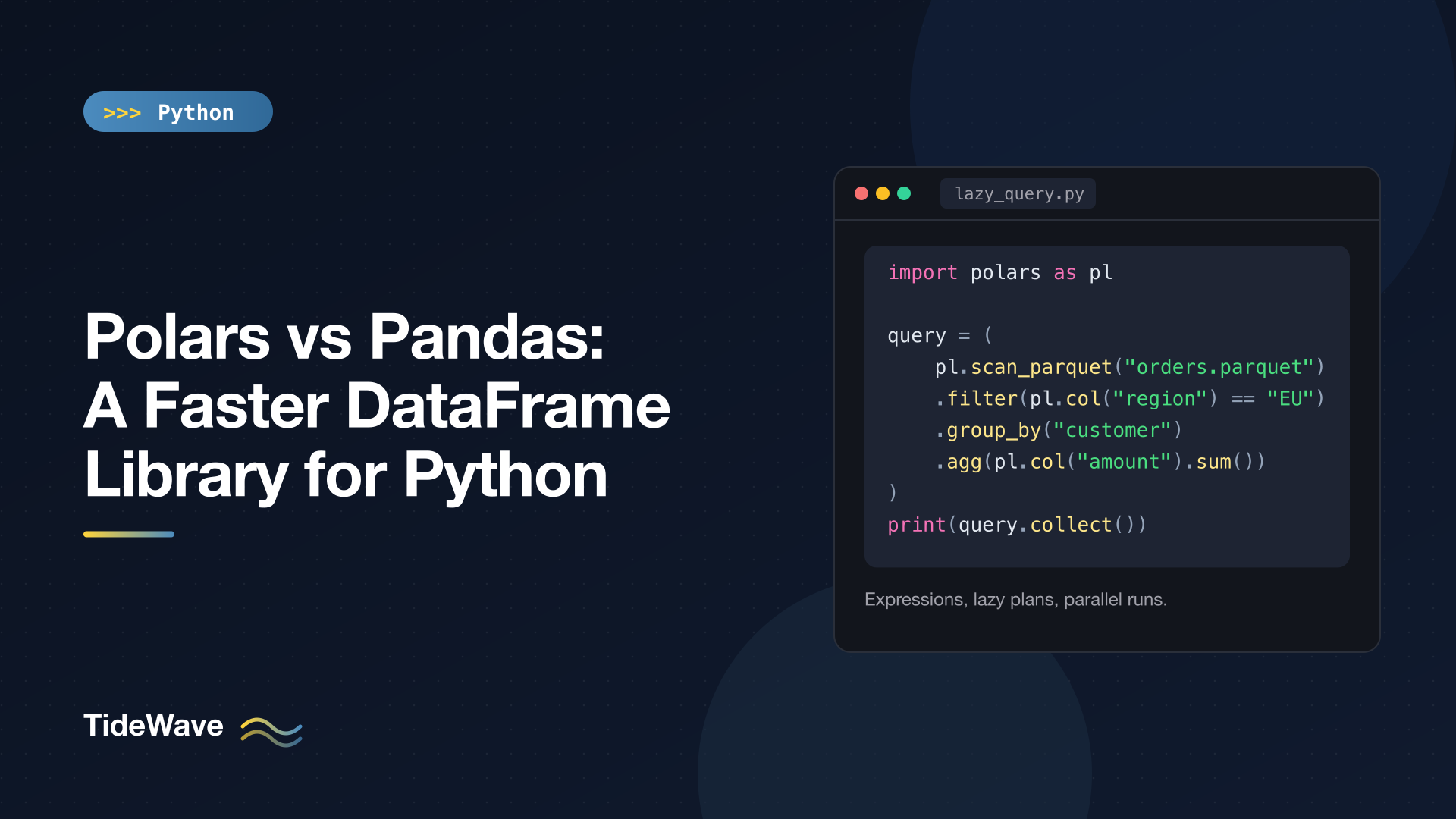
The biggest performance win in Polars comes from the lazy API. Instead of reading a file and operating on it step by step, you scan it, build up a query, and call collect() at the end:

# lazy_query.py
import polars as pl

query = (
    pl.scan_csv("orders.csv", try_parse_dates=True)
    .filter(pl.col("region") == "EU")
    .group_by("customer")
    .agg(pl.col("amount").sum().alias("total"))
    .sort("customer")
)

print(query.explain())
print(query.collect())

explain() shows the optimized plan before anything runs:

SORT BY [col("customer")]
  AGGREGATE[maintain_order: false]
    [col("amount").sum().alias("total")] BY [col("customer")]
    FROM
    simple π 2/2 ["customer", "amount"]
      Csv SCAN [orders.csv]
      PROJECT 3/5 COLUMNS
      SELECTION: col("region") == "EU"
      ESTIMATED ROWS: 8

The plan tells you two important things. PROJECT 3/5 COLUMNS means the CSV reader only parses the three columns the query actually uses (projection pushdown). SELECTION: col("region") == "EU" means the filter is applied while reading, so non-EU rows never get materialized (predicate pushdown). With Parquet files, which store column statistics, Polars can skip entire chunks of the file this way.

pandas has no equivalent. pd.read_csv loads everything you don't explicitly exclude with usecols, and each subsequent step allocates new intermediate DataFrames.

Some guidelines for the lazy API:

Use scan_csv, scan_parquet, or scan_ndjson instead of read_* when working with files.
Call df.lazy() to switch an existing DataFrame into lazy mode.
Call collect() once at the end, not after every step.
For data larger than memory, Polars' streaming engine can process a lazy query in batches: query.collect(engine="streaming").

Performance: What to Expect

Benchmarks depend heavily on the operation, data size, and hardware, so treat any single number with suspicion. Here's a simple script you can run yourself, grouping 10 million rows:

# bench.py
import time

import numpy as np
import pandas as pd
import polars as pl

rng = np.random.default_rng(0)
n = 10_000_000
data = {
    "store": rng.integers(0, 1_000, n),
    "product": rng.integers(0, 5_000, n),
    "amount": rng.uniform(1, 500, n),
}
pdf = pd.DataFrame(data)
pldf = pl.DataFrame(data)


def timed(label, fn):
    start = time.perf_counter()
    fn()
    print(f"{label:<8} {time.perf_counter() - start:.2f}s")


timed("pandas", lambda: pdf[pdf["amount"] > 100]
      .groupby(["store", "product"])["amount"].agg(["sum", "mean", "count"]))
timed("polars", lambda: pldf.filter(pl.col("amount") > 100)
      .group_by("store", "product")
      .agg(
          pl.col("amount").sum().alias("sum"),
          pl.col("amount").mean().alias("mean"),
          pl.len().alias("count"),
      ))

On an 8-core laptop, Polars finished this in roughly a quarter to a half of the pandas time across runs. That's a typical result for in-memory aggregation. The gap usually grows when you read files lazily (pushdown means less I/O), when you have many independent column operations (parallelism), or when you'd otherwise hit pandas' memory overhead from copies.

The gap shrinks, or disappears, for small DataFrames. If your data is a few thousand rows, both libraries finish in milliseconds and the speed difference is irrelevant. Time your actual workload rather than assuming.

Memory and Data Types

Polars stores data in the Apache Arrow columnar format. Strings, dates, nested lists, and missing values all have native, compact representations.

pandas historically stored strings as Python objects, which was slow and memory-hungry. pandas 3.0 changed that: string columns now use a dedicated str dtype by default (backed by PyArrow when it's installed), and Copy-on-Write is always enabled, so chained assignment no longer silently modifies or fails to modify the original. If you learned pandas a few years ago, those two changes remove some of its oldest pain points and narrow the gap.

Missing data is still handled differently:

Polars uses a single null for every type. fill_null, is_null, and drop_nulls work everywhere. NaN is a separate floating-point value, not "missing".
pandas uses NaN for floats, None or NaN in object columns, NaT for datetimes, and pd.NA for nullable extension types. It works, but you need to know which one you're dealing with.

Interoperability

You don't have to choose one library for a whole project. Converting is one call each way:

import polars as pl

pandas_df = orders.to_pandas()      # needs pyarrow
back = pl.from_pandas(pandas_df)

Watch the types when you round-trip. In the example above, the Polars date column comes back from pandas as a Datetime, because pandas stores dates as timestamps. If precise types matter, cast after converting.

This interop is how most teams adopt Polars: use it for the heavy transformations, then hand a pandas DataFrame to the library that expects one (an older plotting tool, a scikit-learn pipeline, a database helper). Some libraries now accept Polars DataFrames directly (Seaborn 0.13, for example, accepts them through the DataFrame interchange protocol), but check before relying on it.

Where pandas Still Wins

Polars isn't a drop-in replacement, and pandas has real advantages:

Ecosystem. statsmodels, many scikit-learn examples, GeoPandas, and countless internal tools assume pandas. Stack Overflow answers, books, and courses overwhelmingly use it.
The index. For time series work with resample, asfreq, and label-aligned arithmetic between Series, the index is a feature, not a burden.
Mutation and quick exploration. Assigning to a single cell, df.loc[row, col] = value, is natural in pandas. Polars DataFrames are effectively immutable; you create new ones.
Familiarity. If your team knows pandas well and your data fits comfortably in memory, the productivity cost of switching might outweigh speed you won't notice.

Where Polars Wins

Speed and memory on medium-to-large data, especially with lazy file scans.
Consistency. A small set of verbs and expressions instead of many overlapping ways to do the same thing (loc, iloc, [], query, where, mask, assign).
Strict types. Errors surface early instead of turning a numeric column into object silently.
Larger-than-memory work via the streaming engine, without reaching for Spark or Dask.
Readable pipelines. Method chains of expressions read like a query, which makes them easier to review.

Making the Decision

A pragmatic way to choose:

Situation	Recommendation
Small data, existing pandas codebase	Stay with pandas
New ETL or data pipeline, files in the GBs	Start with Polars, lazy mode
Heavy time-series resampling	pandas, or Polars `group_by_dynamic` if you're comfortable
A library downstream requires pandas	Polars for transforms, `to_pandas()` at the boundary
Data larger than RAM on one machine	Polars streaming before reaching for a cluster
Teaching beginners, following tutorials	pandas, for the ecosystem of learning material

If you want to try Polars on an existing project, pick the slowest step in a pipeline, rewrite just that step, and compare. That gives you a real measurement and a feel for the API without a risky rewrite.

Conclusion

pandas and Polars solve the same problem with different philosophies. pandas gives you an eager, labeled, flexible DataFrame with an unmatched ecosystem, and pandas 3.0 fixed several long-standing annoyances. Polars gives you strict types, a consistent expression API, automatic parallelism, and a lazy query engine that can skip work entirely.

For small, exploratory work, either is fine and familiarity should decide. For larger data and new pipelines, Polars is often the faster and more predictable choice, and its easy conversion to pandas means you can adopt it one step at a time.