NumPy Fundamentals: Arrays, Broadcasting, and Vectorization

NumPy sits underneath almost all numerical Python. pandas DataFrames store their columns in NumPy-style arrays, scikit-learn takes them as input, Matplotlib plots them, and PyTorch and JAX copied their API. Even if you mostly work with higher-level libraries, understanding NumPy's three core ideas makes everything built on top of it less mysterious: the ndarray (a typed, fixed-size block of numbers), broadcasting (how arrays of different shapes combine), and vectorization (expressing work as whole-array operations instead of Python loops).

This guide covers each of those in turn, with the real output of every example, plus the pitfalls that catch people out: silent integer overflow, views that modify the original array, and broadcasts that succeed when they shouldn't.

The examples were run with NumPy 2.5 on Python 3.13. Install it with python -m pip install numpy, and import it the conventional way:

import numpy as np

Why Not Just Use Lists?

A Python list holds references to separate Python objects, each with its own type information, scattered around memory. Adding two lists of numbers element by element means a Python loop, with type checks and object creation for every element.

A NumPy array is one contiguous block of memory holding raw values of a single type. Operations on it run in compiled C loops over that memory, with no per-element Python overhead. The syntax reflects the difference:

print([1, 2, 3] * 2)
print(np.array([1, 2, 3]) * 2)

[1, 2, 3, 1, 2, 3]
[2 4 6]

For lists, * 2 means repetition. For arrays, arithmetic operators work element-wise. That's the foundation of everything else in this post.

The ndarray

Shape, Dimensions, and dtype

a = np.array([1, 2, 3, 4])
print(a, a.dtype, a.shape, a.ndim)

m = np.array([[1.0, 2.0, 3.0], [4.0, 5.0, 6.0]])
print(m.dtype, m.shape, m.ndim, m.size)

[1 2 3 4] int64 (4,) 1
float64 (2, 3) 2 6

Every array has:

• a dtype, the single type of all its elements (int64, float64, bool, and so on);
• a shape, a tuple giving the length along each dimension (or axis). (4,) is a one-dimensional array of four elements; (2, 3) is two rows and three columns;
• ndim, the number of dimensions, and size, the total number of elements.

When you mix types, NumPy picks a dtype that can hold them all: np.array([1, 2.5, 3]) becomes float64, printed as [1. 2.5 3. ].

Creating Arrays

You'll rarely type arrays out by hand. The common constructors:

np.zeros((2, 3))                 # 2x3 array of 0.0
np.ones(3, dtype=np.int32)       # [1 1 1]
np.full((2, 2), 7)               # 2x2 array of 7
np.arange(0, 10, 2)              # [0 2 4 6 8], like range()
np.linspace(0, 1, 5)             # [0.   0.25 0.5  0.75 1.  ], 5 evenly spaced points
np.eye(3, dtype=int)             # 3x3 identity matrix

arange takes a step size and excludes the end; linspace takes a number of points and includes the end. Prefer linspace for floats, where accumulating a step like 0.1 gives rounding surprises.

For random numbers, create a Generator with default_rng(). It's the modern API, and passing a seed makes results reproducible:

rng = np.random.default_rng(seed=42)
print(rng.integers(1, 7, size=5))              # five dice rolls
print(rng.normal(loc=0, scale=1, size=3).round(3))

[1 5 4 3 3]
[ 0.941 -1.951 -1.302]

Avoid the legacy np.random.seed() / np.random.rand() functions in new code; they share hidden global state.

Reshaping

reshape() changes the shape without changing the data, as long as the total size matches. A -1 means "work this dimension out for me":

x = np.arange(12)
grid = x.reshape(3, 4)
print(grid)
print(x.reshape(2, -1).shape)  # (2, 6)
print(grid.T.shape)            # (4, 3): transpose
print(grid.ravel())            # flatten back to 1-D

[[ 0  1  2  3]
 [ 4  5  6  7]
 [ 8  9 10 11]]

Reshaping is nearly free: it usually returns a view of the same memory with different shape metadata.

dtypes Matter: Overflow and Truncation

Because arrays hold raw machine values, they have machine limits. A Python int grows as large as needed; a NumPy int8 holds −128 to 127, and array arithmetic wraps around silently:

small = np.array([100, 120], dtype=np.int8)
print(small + 100)

[-56 -36]

No error, no warning, wrong answer. The default int64 makes this rare in practice, but it bites with image data (uint8 pixels, 0 to 255), with int32 columns read from files, and when you choose small dtypes to save memory. Convert with astype() before arithmetic that might overflow.

Converting floats to integers truncates toward zero rather than rounding:

print(np.array([1.7, -1.7]).astype(int))  # [ 1 -1]

Use np.round() first if you meant rounding. On the plus side, choosing dtypes deliberately is a powerful memory tool: one million float32 values take 4 MB instead of 8 MB for float64.

Indexing and Slicing

Basic Indexing

Arrays index like nested lists, but with one comma-separated index per axis:

grid = np.arange(12).reshape(3, 4)

grid[1, 2]      # 6: row 1, column 2
grid[0]         # [0 1 2 3]: first row
grid[:, 1]      # [1 5 9]: second column
grid[1:, ::2]   # rows 1 onward, every other column
grid[-1, -1]    # 11: last element

grid[1:, ::2] gives:

[[ 4  6]
 [ 8 10]]

grid[:, 1] (all rows, column 1) is the kind of selection that's awkward with nested lists and trivial here.

Slices Are Views

This is the most important difference from lists. Slicing a list copies it. Slicing an array returns a view: a new array object that shares memory with the original. Writing through the view changes the original:

row = grid[0, :2]
row[0] = 99
print(grid[0])
print(np.shares_memory(row, grid))

[99  1  2  3]
True

Views make slicing fast and memory-cheap, even on huge arrays. When you need an independent array, say so explicitly with .copy():

safe = grid[0, :2].copy()
safe[0] = -1          # grid is unaffected

Boolean Masks

A comparison produces a boolean array of the same shape, and indexing with it selects the matching elements:

temps = np.array([18.5, 22.1, 25.3, 19.8, 30.2, 27.6])
hot = temps > 25
print(hot)
print(temps[hot])
print(temps[(temps > 20) & (temps < 28)])
print(hot.sum(), hot.mean())

[False False  True False  True  True]
[25.3 30.2 27.6]
[22.1 25.3 27.6]
3 0.5

As in pandas (which inherited this from NumPy), combine conditions with &, |, ~, and wrap each in parentheses. Summing a boolean array counts the True values, and its mean is the fraction that are True: three hot days, 50% of the readings.

Masks also work on the left of an assignment, which replaces values in place:

temps[temps > 28] = 28   # cap outliers

Fancy Indexing

Indexing with a list or array of integers picks elements by position, in any order:

print(temps[[0, 2, 4]])        # [18.5 25.3 30.2]

order = np.argsort(temps)      # positions that would sort the array
print(order, temps[order])

[0 3 1 2 5 4] [18.5 19.8 22.1 25.3 27.6 30.2]

Unlike slices, boolean and fancy indexing return copies. Modifying temps[[0, 2]] after extracting it doesn't touch temps. The rule of thumb: slices (start:stop:step) give views; anything indexed by arrays gives copies.

np.where and Friends

np.where(condition, a, b) is a vectorized if/else, choosing from a where the condition holds and b elsewhere:

print(np.where(temps > 25, "hot", "ok"))
print(np.where(temps > 25)[0])   # with one argument: the matching indices
print(np.clip(temps, 20, 28))    # bound values to a range

['ok' 'ok' 'hot' 'ok' 'hot' 'hot']
[2 4 5]
[20.  22.1 25.3 20.  28.  27.6]

Universal Functions and Aggregations

Element-wise Math

Universal functions (ufuncs) apply an operation element by element in compiled code. Arithmetic operators are ufuncs, and NumPy has dozens more: np.sqrt, np.exp, np.log, np.sin, np.abs, np.maximum, np.minimum, and so on:

a = np.array([1.0, 4.0, 9.0, 16.0])
print(a + 10)           # [11. 14. 19. 26.]
print(np.sqrt(a))       # [1. 2. 3. 4.]
print(np.maximum(a, 5)) # [ 5.  5.  9. 16.]

Use these instead of the math module's functions, which only accept single numbers.

Aggregating Along an Axis

Reductions like sum, mean, min, max, std, argmax, cumsum collapse an array. By default they reduce everything; the axis argument picks which dimension to collapse:

sales = np.array([
    [120, 95, 130],   # store A: Jan, Feb, Mar
    [80, 110, 90],    # store B
    [150, 160, 170],  # store C
])

print(sales.sum())                 # everything
print(sales.sum(axis=0))           # collapse rows -> one total per month
print(sales.sum(axis=1))           # collapse columns -> one total per store
print(sales.mean(axis=1).round(1))
print(sales.argmax(axis=1))        # best month index for each store

1105
[350 365 390]
[345 280 480]
[115.   93.3 160. ]
[2 1 2]

The way to remember axis: it's the dimension that disappears. sales has shape (3, 3) as (stores, months). axis=0 removes the stores dimension, leaving one value per month; axis=1 removes months, leaving one value per store.

keepdims=True keeps the collapsed axis with length 1, which turns out to be exactly what broadcasting needs:

print(sales.sum(axis=1, keepdims=True))

[[345]
 [280]
 [480]]

Broadcasting

Element-wise operations are easy when both arrays have the same shape. Broadcasting is the set of rules NumPy uses when they don't: it virtually stretches the smaller array to match the larger one, without actually copying data.

You've already used the simplest case. In sales * 1.1, the scalar is broadcast against every element.

The Rules

To combine two arrays, NumPy compares their shapes from the right, dimension by dimension. Two dimensions are compatible if they're equal, or one of them is 1. If one array has fewer dimensions, it's treated as if it had extra length-1 dimensions on the left. Length-1 dimensions are stretched to match.

Shape A	Shape B	Result	Why
(3, 3)	() (scalar)	(3, 3)	Scalar stretches everywhere
(3, 3)	(3,)	(3, 3)	(3,) is treated as (1, 3): one row, repeated for every row
(3, 3)	(3, 1)	(3, 3)	One column, repeated for every column
(3, 1)	(1, 4)	(3, 4)	Both stretch: an "outer" combination
(3, 3)	(2,)	Error	3 vs 2: neither equal nor 1

A Row Across Every Row

Suppose each month has a different unit price. A 1-D array of three prices lines up with the last axis (months) and is applied to every store:

price = np.array([2.0, 2.5, 3.0])  # per-month price
print(sales * price)

[[240.  237.5 390. ]
 [160.  275.  270. ]
 [300.  400.  510. ]]

A Column Across Every Column

To apply one value per store instead, you need a column: shape (3, 1), not (3,):

store_target = np.array([[100], [100], [150]])
print(sales - store_target)

[[ 20  -5  30]
 [-20  10 -10]
 [  0  10  20]]

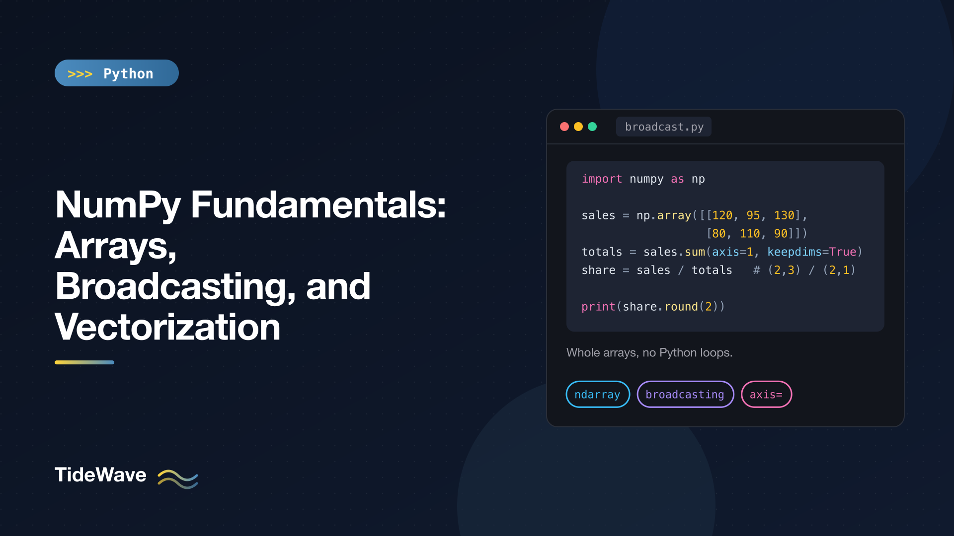
That's where keepdims=True earns its keep. Each store's share of its own quarterly total:

share = sales / sales.sum(axis=1, keepdims=True)
print(share.round(2))

[[0.35 0.28 0.38]
 [0.29 0.39 0.32]
 [0.31 0.33 0.35]]

Each row now sums to 1.

The Silent Broadcasting Bug

What if you forget keepdims? sales.sum(axis=1) has shape (3,), which broadcasts as a row, so each column is divided by a different store's total:

wrong = sales / sales.sum(axis=1)
print(wrong.round(2))

[[0.35 0.34 0.27]
 [0.23 0.39 0.19]
 [0.43 0.57 0.35]]

No error. Because the array is square, the shapes happen to be compatible, and you get plausible-looking nonsense. On a non-square array the same mistake would raise an error. The defense: think about which axis a 1-D array lines up with (always the last one), use keepdims=True or explicit (n, 1) shapes for per-row values, and check .shape when in doubt.

When shapes truly are incompatible, the error tells you exactly what didn't match:

sales + np.array([1, 2])
# ValueError: operands could not be broadcast together with shapes (3,3) (2,)

Adding Axes with np.newaxis

You can insert a length-1 axis with None (or its alias np.newaxis) to set up a broadcast deliberately. Combining a column with a row produces every pairwise combination, a multiplication table here:

x = np.arange(1, 4)
print(x[:, np.newaxis] * x)

[[1 2 3]
 [2 4 6]
 [3 6 9]]

x[:, np.newaxis] has shape (3, 1) and x has shape (3,), treated as (1, 3), so the result is (3, 3).

The same idea computes all pairwise distances between points without a single loop:

points = np.array([[0.0, 0.0], [3.0, 4.0], [6.0, 8.0]])
diff = points[:, None, :] - points[None, :, :]   # shape (3, 3, 2)
dist = np.sqrt((diff ** 2).sum(axis=-1))
print(dist)

[[ 0.  5. 10.]
 [ 5.  0.  5.]
 [10.  5.  0.]]

A (3, 1, 2) array minus a (1, 3, 2) array gives every point-minus-point difference; squaring, summing over the last axis, and taking the square root gives the Euclidean distances. Be aware that this creates an (n, n, d) intermediate array, which gets large quickly; for big inputs, use scipy.spatial.distance.cdist.

A classic everyday use is standardizing columns (subtracting each column's mean and dividing by its standard deviation), which broadcasts a (n_columns,) row of statistics over every row:

data = np.array([[1.0, 200.0], [2.0, 300.0], [3.0, 400.0]])
z = (data - data.mean(axis=0)) / data.std(axis=0)
print(z.round(3))

[[-1.225 -1.225]
 [ 0.     0.   ]
 [ 1.225  1.225]]

Vectorization: Replacing Loops

Vectorization means expressing a computation as operations on whole arrays, so the looping happens in compiled code rather than in Python. It's the main reason to use NumPy at all.

How Big Is the Difference?

Here's an order total computed with a Python loop and with NumPy:

# vectorize_bench.py
import math
import timeit

import numpy as np

rng = np.random.default_rng(0)
prices = rng.uniform(1, 100, size=1_000_000)
quantities = rng.integers(1, 10, size=1_000_000)
prices_list = prices.tolist()
quantities_list = quantities.tolist()


def total_loop(prices: list[float], quantities: list[int]) -> float:
    total = 0.0
    for p, q in zip(prices, quantities):
        total += p * q
    return total


def total_numpy(prices: np.ndarray, quantities: np.ndarray) -> float:
    return float((prices * quantities).sum())


print(math.isclose(total_loop(prices_list, quantities_list), total_numpy(prices, quantities)))

loop = min(timeit.repeat(lambda: total_loop(prices_list, quantities_list), number=5, repeat=3)) / 5
vec = min(timeit.repeat(lambda: total_numpy(prices, quantities), number=5, repeat=3)) / 5
print(f"loop:  {loop * 1000:.1f} ms")
print(f"numpy: {vec * 1000:.1f} ms")
print(f"speedup: {loop / vec:.0f}x")

On my machine:

True
loop:  28.9 ms
numpy: 0.8 ms
speedup: 35x

Your numbers will differ, but a 10x to 100x gap is typical for simple arithmetic. (The loop gets plain Python lists, its best case; looping over a NumPy array element by element is even slower, because each element has to be boxed into a Python object.) For more on measuring this kind of thing properly, see profiling Python code with cProfile and timeit.

Vectorizing Conditional Logic

Loops with if/elif branches look hard to vectorize, but they map onto np.where (two branches) or np.select (several). A tiered shipping cost:

def shipping_loop(weights: list[float]) -> list[float]:
    out = []
    for w in weights:
        if w <= 1:
            out.append(5.0)
        elif w <= 10:
            out.append(5.0 + (w - 1) * 1.5)
        else:
            out.append(20.0 + (w - 10) * 1.0)
    return out


def shipping_vec(weights: np.ndarray) -> np.ndarray:
    return np.select(
        [weights <= 1, weights <= 10],
        [5.0, 5.0 + (weights - 1) * 1.5],
        default=20.0 + (weights - 10) * 1.0,
    )


w = np.array([0.5, 1.0, 4.0, 10.0, 25.0])
print(shipping_vec(w))

[ 5.   5.   9.5 18.5 35. ]

np.select checks the conditions in order and takes the value from the first one that's true, exactly like the if/elif chain. On a million weights, the loop took 76 ms and the vectorized version 6.1 ms on my machine.

Note that the vectorized version computes every branch for every element and then picks. That's usually still far faster, but it means a branch that would raise an error or warning for some inputs (like np.log of zero) gets evaluated on them anyway.

np.vectorize Is Not Vectorization

np.vectorize looks like it should speed up a Python function, but the documentation is explicit that it's essentially a for loop provided for convenience. In my test it ran the shipping logic in about the same time as the plain loop. Use it for convenience (broadcasting a scalar function over arrays), not for speed.

Thinking in Arrays

A few patterns cover most loop conversions:

Loop pattern	Vectorized version
Running total	np.cumsum(a)
Running product (e.g. compound growth)	np.cumprod(1 + rates)
Difference from previous element	np.diff(a)
Count matching items	(a > threshold).sum()
If/else per element	np.where(cond, x, y)
Several branches	np.select(conditions, choices, default)
Look up values by code	Fancy indexing: table[codes]
Pairwise combinations	Broadcasting with [:, None]

When none of these fit, and the logic genuinely depends on the previous iteration's result in a complex way, a loop may be the right tool. That's when people reach for Numba or Cython to compile the loop itself; see speeding up Python code for those options.

Common Pitfalls

• Unexpected views. Modifying a slice modifies the original. Call .copy() when you need independence.
• Silent overflow with small integer dtypes. Check dtype on data you didn't create.
• Wrong-axis broadcasting on square arrays. Use keepdims=True and check shapes.
• Floating-point comparisons. 0.1 + 0.2 == 0.3 is False in NumPy too. Use np.isclose() or np.allclose().
• Growing arrays in a loop. np.append copies the whole array every time. Collect values in a list and convert once, or preallocate with np.empty() and fill.
• and/or on arrays raise "The truth value of an array with more than one element is ambiguous". Use &, |, and parentheses.

Conclusion

NumPy's power comes from three ideas working together. The ndarray stores numbers of one dtype in contiguous memory, which makes operations fast but means you should pay attention to dtypes and to the difference between views and copies. Broadcasting lets arrays of different shapes combine by comparing shapes from the right and stretching length-1 dimensions. And vectorization means writing computations as whole-array expressions (ufuncs, reductions along an axis, masks, np.where, np.select) so the loops run in compiled code. Once these click, pandas, scikit-learn and the rest of the scientific Python stack start to feel like natural extensions; pandas DataFrames: filtering, grouping, and merging is a good next step.